In Brief
An analysis by MIT researchers shows that when electric power companies are planning to invest in new generating facilities but face the possibility of future limits on carbon emissions, they can reduce their long-term economic risk by having at least 20% of the new generation come from non-carbon systems such as solar and wind. Coal or natural gas plants are less expensive initially, but they might have to be shut down prematurely if a carbon cap is put in place in the coming decades. Non-carbon systems are more costly to build, but they’re relatively inexpensive to operate, so companies will continue to run them, even if there’s no restriction on carbon emissions. The researchers’ novel method of incorporating expectations about future emissions policies into the decision-making process identifies an investment strategy that can as much as halve cumulative costs to the US economy, potentially saving more than $100 billion over the long term.
When planners in an electric power company need to add new generating capacity, they may consider building a plant that burns coal or natural gas. After all, such fossil fuel–fired facilities are relatively inexpensive and should run for 40 years or more. But if future policies impose strict limits on carbon emissions, they might need to shut down their fossil fuel plants and build non-carbon systems such as solar or wind in a hurry—two extremely expensive propositions. On the other hand, if they build the more expensive non-carbon systems now and emissions policies aren’t enacted, they may have spent that extra money unnecessarily. Deciding to build fossil plants or choosing to invest in non-carbon generation—either decision has economic risk, given the uncertainty about long-term emissions policy.
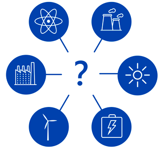
Power company planners can choose from a variety of technologies, as suggested in this illustration. But comparing costs is tricky. While the present cost of building a facility may be known, any climate policy enacted during its lifetime can significantly impact the long-term value of the initial investment. Graphic: Jenn Schlick, MITEI
To help with such decision making, planners often use modeling tools that identify the best option based on various assumptions about the future. For example, one model may assume that today’s conditions will continue; another may assume perfect foresight of how the future will unfold; and yet another may call for analyzing different possible scenarios and then picking one—most likely the one in the middle. “But an important piece that’s often left out is explicit consideration of uncertainty, often because it can be difficult to incorporate or even to characterize that uncertainty, much less how it should impact your decision,” says Jennifer Morris SM ’09, PhD ’13, a research scientist in the MIT Joint Program on the Science and Policy of Global Change and the MIT Energy Initiative.
For the past five years, Morris and her Joint Program colleagues—John Reilly, co-director of the Joint Program and a senior lecturer at the Sloan School of Management; Mort Webster, former MIT associate professor of engineering systems and now associate professor of energy engineering at Pennsylvania State University; and Vivek Srikrishnan, a PhD candidate at Pennsylvania State University—have been developing an approach that explicitly incorporates uncertainty into the decision-making process. “You don’t know exactly how the future is going to unfold, but you have an idea—you have an expectation—of the probability of different futures,” says Morris. “Our goal is to enable you to use that long-term expectation to inform what action you should take now.”
Modeling the economy
At the core of their approach is a computable general equilibrium (CGE) model—a type of simulation that tracks the flows of goods and services and the corresponding monetary flows among all sectors of the US economy. “Enactment of a climate policy will affect all sectors, and by using a CGE model, we can track ripple effects throughout the economy and measure the economy-wide impacts,” says Morris.
Performing an uncertainty analysis can require running tens of thousands of simulations, so for this study Morris developed a simplified CGE model that captures key sectors, among them electric power, and uses aggregated US data. She included two types of electricity generation—conventional fossil (coal and natural gas) and a generalized non-carbon electricity (wind, solar, advanced nuclear, and carbon capture and storage). She assumed an aggregate cost for the non-carbon electricity sources that’s 50% higher than the cost of conventional sources. Why such a high cost? “Our CGE model looks at system costs,” she explains. “Once we account for the variability and intermittency of renewable power generation and the need for backup capacity or storage and additional transmission and distribution, the current systemwide cost of the non-carbon options comes out that much higher.”
The optimal investment choice is defined as the one that will minimize costs and thereby maximize welfare in all economic sectors over two time periods—now (when the decision is being made) and later (when a policy has—or hasn’t—been enacted). To factor in the uncertainty of future policy, Morris put the CGE model into a dynamic programming framework and then defined two time periods for analysis—2010 to 2020 and 2020 to 2030. This two-stage framework determines the overall welfare effect by calculating the cost in the first stage plus the expected cost in the second stage.
Defining policy expectations
To perform an analysis, Morris first defines quantitatively a range of expectations about the most likely policy action in the future. The figure below shows four examples, presented as probability density functions, or PDFs. The X-axis shows possible second-stage emissions caps reported as percent reductions in cumulative emissions from the electric power sector from 2015 to 2030 below a reference scenario that assumes no limits on emissions. Thus, 100% indicates that no new emissions cap is expected in 2020, 80% foresees a policy that calls for cutting emissions by 20%, and so on.
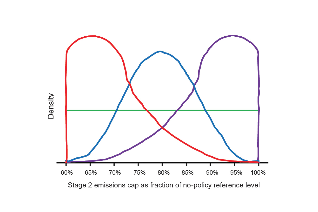
Expectations about emissions policy actions in the future The illustrative probability density functions (PDFs) presented above define four sets of expectations about the likelihood of emissions caps at varying levels being enacted in the future. The reference case is defined as 100%, meaning that there’s no cap on emissions. Other caps are presented as percentages of that reference level (e.g., 80% means a 20% reduction relative to reference emissions). The farther left on the X-axis, the tighter the emissions cap; the higher the curve at a given cap, the more likely that cap is believed to be. The horizontal line represents the expectation that all emissions caps are equally likely in the future.
Each PDF shows a different view of how likely those values are. The horizontal line represents the view that all possible emissions caps are equally likely in the future. In the other examples, the highest point is the value deemed most likely—the one receiving the most votes, if you will—and the lowest point is the value seen as least likely. Accordingly, the familiar bell curve deems the middle caps most likely and the more extreme policies (unrestricted emissions and severely constrained emissions) unlikely. In the other two curves, the highest section is skewed toward the right or toward the left, indicating that future emissions are more likely to be unre-stricted or more likely to be severely constrained.
Given a single PDF, the simplest approach would be to pick the highest point—thus the future cap deemed most likely—and determine the best level of non-carbon investment accordingly. But while the highest point is the most likely future cap, there’s still some chance that the cap could end up elsewhere—maybe even on the tails of the curve reflecting a strict policy or no policy at all. Morris’s modeling system takes all of the possible outcomes into account, weighting the levels according to their likelihood.
To identify the optimal non-carbon investment decision for a given PDF, the system first draws random samples from the possible second-stage policy caps. Because of the sampling method used, more of the selected samples will be the caps deemed most probable, but at least some will be “less likely” points on the tails of the curve.
The system then considers one possible investment level—say, 5% non-carbon generation—and calculates economy-wide consumption over the two time periods for each randomly selected sample. It then considers another investment level and performs the same calculation. By examining many investment levels, it identifies the one that maximizes welfare for the policy expectations represented by that PDF.
Using that procedure, the researchers identified the optimal non-carbon investment level that maximizes welfare under a series of PDFs. Remarkably, they found substantial overlap between the best investment choices. For most of the PDFs they considered, the optimal investment in non-carbon generation was between 20% and 30%. And if the costs of non-carbon alternatives were lower, then an even higher level of investment in non-carbon generation would be optimal.
“So the main takeaway of our study is that the risk of underinvesting in non-carbon generation is far greater than the risk of overinvesting,” says Morris. Why the imbalance? If a company doesn’t have enough non-carbon generation in place to meet strict emissions limits, it will incur high costs as it both abandons its existing fossil systems and rushes to build new non-carbon capacity—without prior experience and knowledge. In contrast, if a company has built non-carbon systems, it will continue to use them regardless of future policy action or inaction because the cost of operating them is low. “So fossil capital is shut down under tight caps, but non-carbon capital is never abandoned under loose caps,” says Morris. “It’s never economic to leave non-carbon generating capital unused.” As an added benefit, early investment in non-carbon technologies enables a company to develop the capacity and the infrastructure needed to scale up non-carbon generation quickly if a much higher share is needed in subsequent decades.
Benefits of optimal analysis
How do Morris’s results compare with results from using other strategies to determine the best investment level? To find out, she looked at three other common approaches. “Deterministic” assumes that the most likely value of the PDF will be the certain outcome and calculates the best investment based on that assumption; “myopic” doesn’t consider the future but just responds to present conditions; and “aggressive” seeks to avoid the worst possible outcome so in this case calls for a high level of non-carbon investment. Using each of those decision strategies, Morris calculated the best first-stage investment decision. While the optimal strategy results in 20% investment in non-carbon generation, the deterministic and myopic both end up with 5% and the aggressive with 50%.
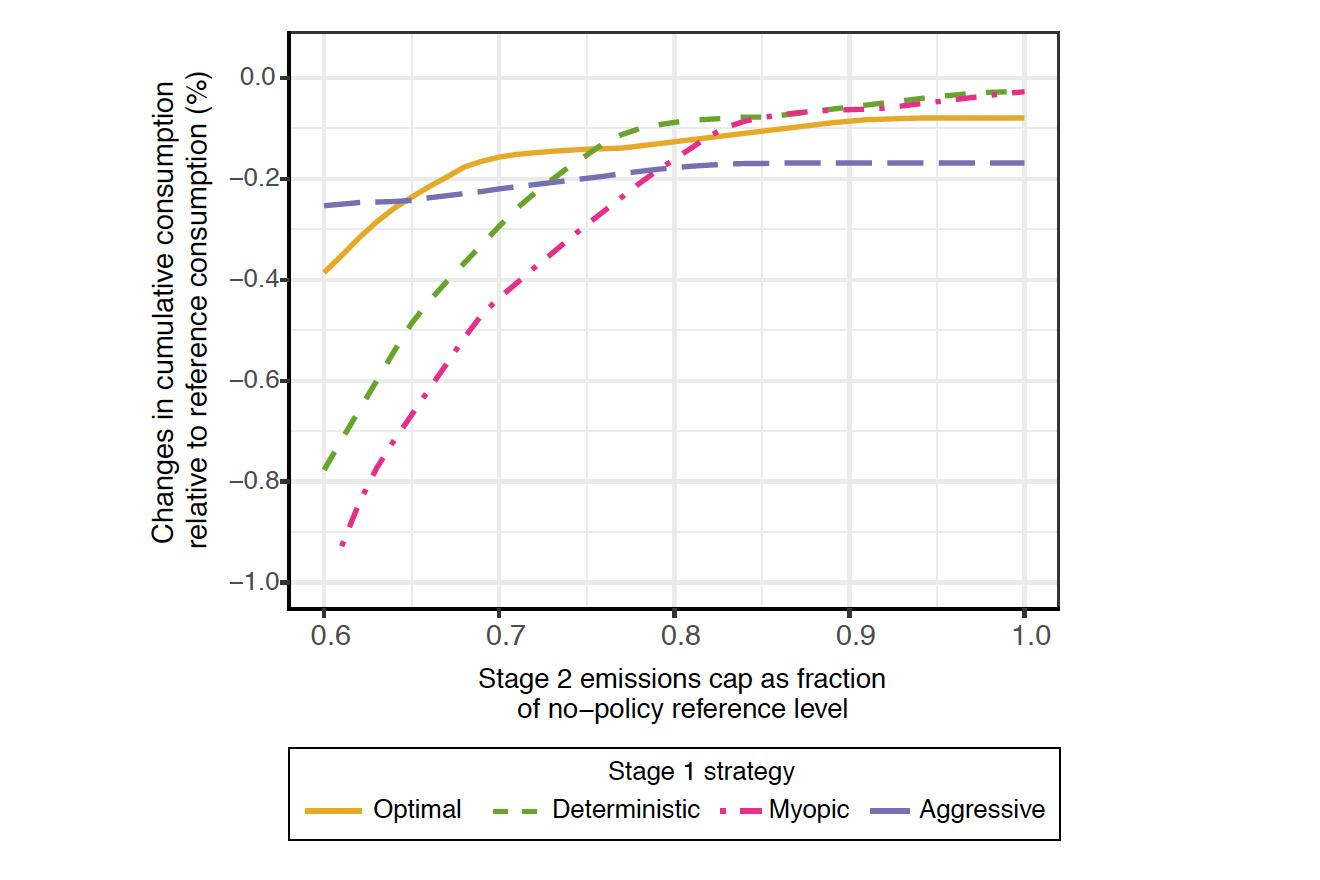
Cumulative economy-wide cost under different investment strategies These curves show the cost—defined as the change in cumulative economy-wide consumption (2010–2030) relative to the reference no-policy consumption level—at various levels of second-stage emissions caps based on first-stage investment choices made using four decision-making strategies. The aggressive approach, which calls for high non-carbon investment, does better than the other strategies if the second-stage cap is stringent. The optimal strategy does well under all but the most stringent emissions caps, while the deterministic and myopic approaches do best when caps are more lenient or non-existent.
For each of those four outcomes, Morris performed CGE simulations to determine the likely impacts on cumulative cost (2010–2030) at different levels of a second-stage emissions cap. Results appear in the figure above. If the second-stage cap is stringent (toward the left in the diagram), the deterministic and myopic approaches bring large welfare losses. The optimal decision cuts off most of those losses, while the aggressive strategy is most successful—a result of its risk-averse high investment in non-carbon generation. As the emissions cap becomes less stringent, costs under the optimal decision quickly decrease and then level off; and after a considerable lag, the deterministic and myopic decisions do the same. The aggressive approach protects against the worst-case loss at strict emissions caps but otherwise costs more than the other strategies.
The figure below also shows how costs under the four strategies are affected by the need to shut down existing generating capacity in order to meet newly imposed emissions caps. The costs here include any system—fossil or non-carbon—that must be scrapped. The most striking result is that the aggressive strategy never incurs costs for unused capital. In contrast, when emission caps are stringent, the deterministic and myopic strategies—and to some extent the optimal strategy—incur high costs for fossil generating capacity they can’t use. As the cap eases, the cost of unused capital drops to zero. Even though all the strategies call for some level of investment in non-carbon generation, the systems that are built never turn into costly unused capital.
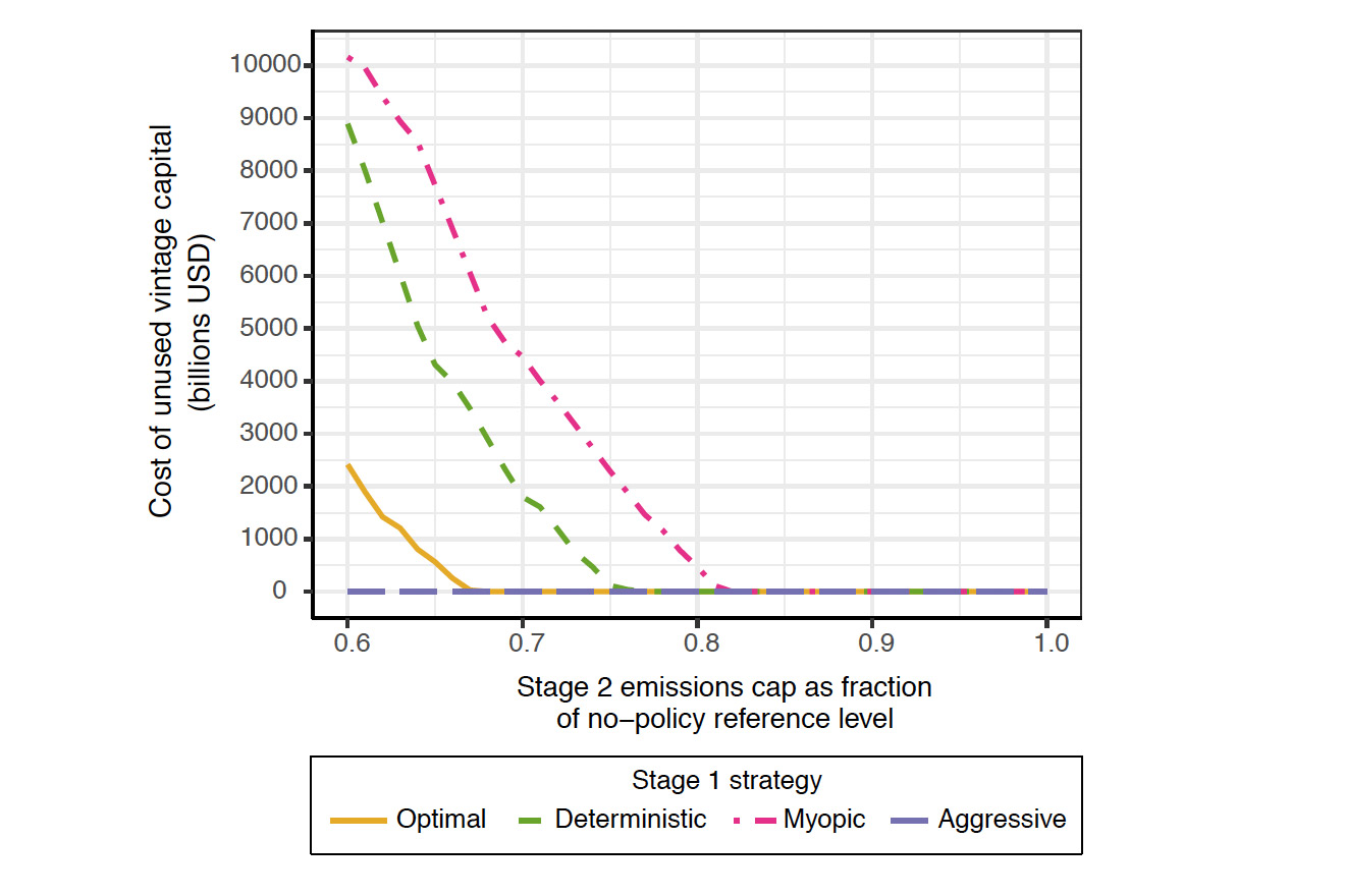
Cost of unused capital as a function of second-stage cap These curves show the cost of capital equipment—both fossil and non-carbon—that must be scrapped under the four decision-making strategies at various second-stage caps. The costs under the optimal, deterministic, and myopic strategies reflect fossil generating capacity that can’t be used when emissions caps are tight. Under looser caps, the cost of unused capital drops to zero because those fossil systems no longer must be abandoned and any non-carbon systems will continue to run. The aggressive strategy incurs no cost from unused capital because the non-carbon generating equipment is never shut down.
Morris recognizes that her analytical approach requires more effort and far more computer time than other commonly used methods of decision making. To measure the value of including uncertainty, Morris looked at total long-term costs associated with sample results from the four techniques. Under one set of assumptions, the expected overall cost to the US economy of using the optimal approach was $150 billion. Costs were 53% higher with the deterministic approach, 109% higher with the myopic strategy, and 23% higher with the aggressive approach. The percentage added cost varied under different assumptions, as shown in the figure below, but it was always higher. “So the incremental cost of choosing a non-optimal investment strategy by explicitly neglecting uncertainty can be significant,” says Morris.
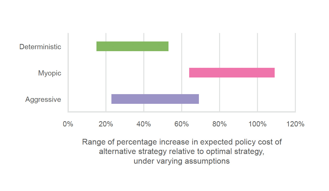
Expected value of including uncertainty To test the value of explicitly incorporating uncertainty, the researchers calculated the total long-term costs of investment choices determined by the four strategies under a variety of assumptions. This figure shows percentage increases in those costs as a result of using the deterministic, myopic, or aggressive strategies rather than the optimal strategy. While the percentage increase varies with the assumptions used, the optimal strategy always does best.
Good news—but new challenges
Morris notes that over the last decade, about 19% of new US power generation has come from non-carbon systems. “So the good news is that the industry has been on track with what our study shows is the optimal amount of investment,” says Morris. “A question for the next decade is, are we going to be able to maintain and even increase that pace?”
Past growth in non-carbon generation has taken place while policies such as production tax credits for renewables and other statewide initiatives were in place. But some of those incentives are going to expire soon. In addition, the current US administration has pulled out of the Paris Agreement, challenged the Clean Power Plan, and taken other steps that are inconsistent with encouraging investment in non-carbon generation.
“Should the current administration’s decisions impact your optimal near-term investment in non-carbon generation?” asks Morris. “Only to the extent that you believe they’re going to persist through the next 30 to 40 years—the lifetime of your investment. If you think that in the next four to eight years we’re going to get back on track and rejoin the global effort to confront climate change, then you should continue with the optimal investment choice, putting 20% or more of your investment dollars into non-carbon sources.”
Notes
This research was supported by the US Department of Energy, Office of Science; the US Environmental Protection Agency; the National Science Foundation; and other government, industry, and foundation sponsors of the Joint Program on the Science and Policy of Global Change (for a list of Joint Program sponsors, see globalchange.mit.edu/sponsors/all). Further information can be found in:
J. Morris, V. Srikrishnan, M.D. Webster, and J.M. Reilly. “Hedging strategies: Electricity investment decisions under policy uncertainty.” The Energy Journal, 2018. Preprint online at www.iaee.org/en/publications/ejarticle.aspx?id=3028.
J. Morris, M. Webster, and J. Reilly. Electricity Generation and Emissions Reduction Decisions under Policy Uncertainty: A General Equilibrium Analysis. Joint Program Report No. 260, April 2014. Online at globalchange.mit.edu/publication/15786.
J. Morris, M. Webster, and J. Reilly. Electricity Investments under Technology Cost Uncertainty and Stochastic Technological Learning. Joint Program Report No. 297, May 2016. Online at globalchange.mit.edu/publication/16200.
This article appears in the Autumn 2017 issue of Energy Futures.